Step-by-Step Guide: Analyzing Microarray Data in Bioconductor
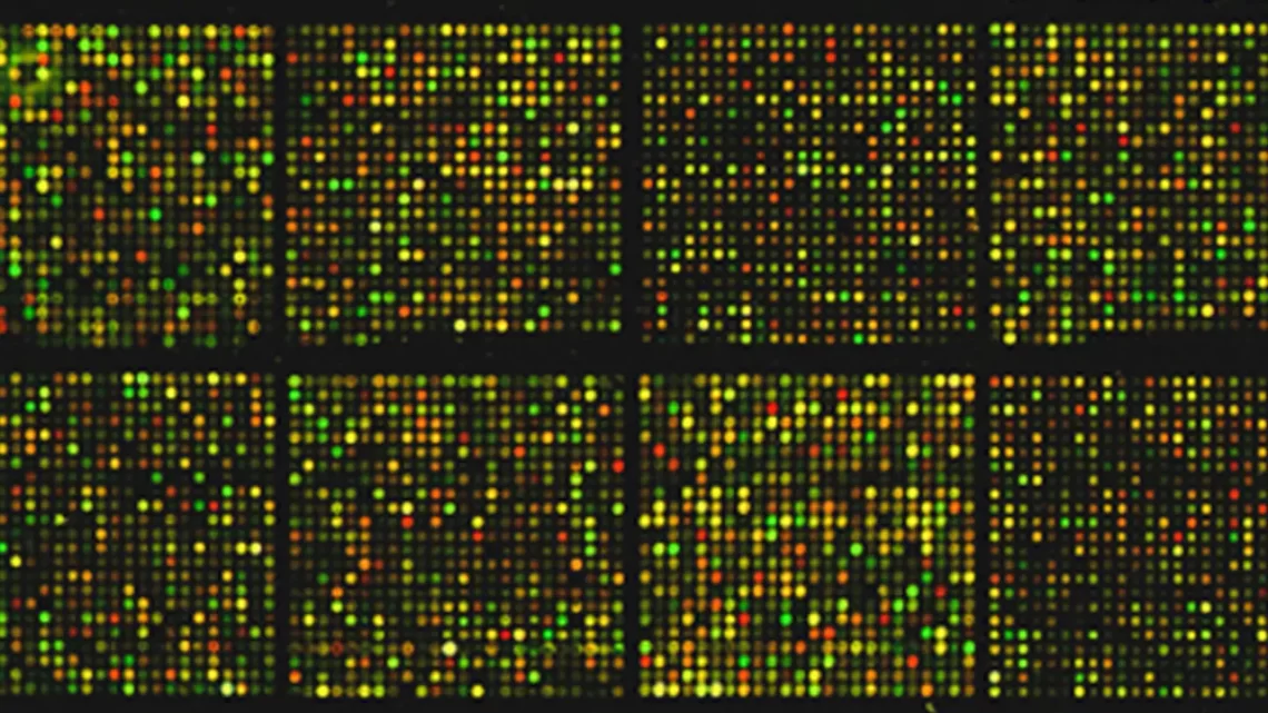
December 28, 2024Microarray data analysis is an essential task in bioinformatics, often used to examine gene expression patterns. Bioconductor, an open-source software project, provides tools for analyzing high-throughput genomic data, including microarrays. Below is a beginner-friendly guide to help you perform microarray data analysis using Bioconductor.
1. Install Necessary Bioconductor Packages
To get started with microarray data analysis in Bioconductor, we need to install the required packages. These packages will allow you to load, normalize, and annotate your microarray data.
2. Load Libraries
Once the packages are installed, you need to load them into your R environment.
3. Set Working Directory and Download Data
You’ll need to set a working directory where the data will be stored and then download the raw CEL files from GEO (Gene Expression Omnibus). For this tutorial, we’ll use a sample dataset identified by the GEO accession ID “GSE27447”.
4. Unpack the CEL Files
Once the CEL files are downloaded, unpack them to access the raw data.
5. Read Raw Data
Now that we have the CEL files, we can load them into R using the ReadAffy function.
6. Normalize the Data
Normalization is essential for removing systematic biases in microarray data. The most common normalization methods are RMA (Robust Multi-array Average) and GCRMA. For this tutorial, we’ll use RMA normalization.
7. Map Probe Sets to Gene Symbols and IDs
Microarrays typically use probe sets that correspond to gene features. You can map these probe sets to gene symbols and Entrez IDs using Bioconductor annotation packages.
8. Save the Data
After annotation, you can save the results to a text file for further analysis or sharing with collaborators.
9. Visualize the Data (Optional)
To interpret the results, visualization is key. A common way to visualize gene expression data is through heatmaps. You can use the heatmap.2 function from the gplots package for this purpose.
10. Differential Expression Analysis (Optional)
If you’re interested in finding differentially expressed genes between conditions, you can use packages such as limma or DESeq2. Below is a basic example using limma for linear modeling.
Applications of Microarray Data Analysis in Bioinformatics:
- Gene Expression Profiling: Microarrays are widely used to study gene expression across different biological conditions.
- Disease Biomarkers: Identifying differentially expressed genes as potential biomarkers for diseases such as cancer, diabetes, and cardiovascular diseases.
- Gene Function: Analyzing gene expression data to understand the function of unknown genes.
- Pathway Analysis: Identifying biological pathways affected by specific conditions or treatments.
Why is Microarray Data Analysis Important?
Microarray analysis allows researchers to study thousands of genes simultaneously, providing valuable insights into gene regulation and biological processes. It is essential in understanding diseases, discovering new therapeutic targets, and advancing precision medicine.
Conclusion
In this tutorial, we’ve covered the basics of analyzing microarray data using Bioconductor. We’ve gone from installing necessary packages, downloading and processing raw data, performing normalization, annotating probes, and visualizing the results. For beginners, this guide should provide a strong foundation for starting microarray data analysis. As you progress, you can explore more advanced techniques like differential expression analysis and pathway enrichment.


