Database Management Systems for Bioinformatics
March 30, 2024 Off By adminCourse Description and Objectives: This course provides an introduction to database management systems (DBMS) with a focus on organizing, maintaining, and retrieving data efficiently from a relational database in the context of bioinformatics. It covers requirements gathering, conceptual, logical, and physical database design, SQL query language, query optimization, and transaction processing. The course aims to equip students with the skills necessary to design and manage databases effectively for bioinformatics applications.
Table of Contents
ToggleDatabases and Database Users
Introduction to databases and DBMS approach in bioinformatics
Databases play a crucial role in bioinformatics, where vast amounts of biological data are generated, stored, and analyzed. In this field, databases serve as repositories for various types of biological data, such as genomic sequences, protein structures, gene expression profiles, and metabolic pathways. The efficient management of these databases is essential for facilitating data access, integration, and analysis, which are critical for advancing research in bioinformatics.
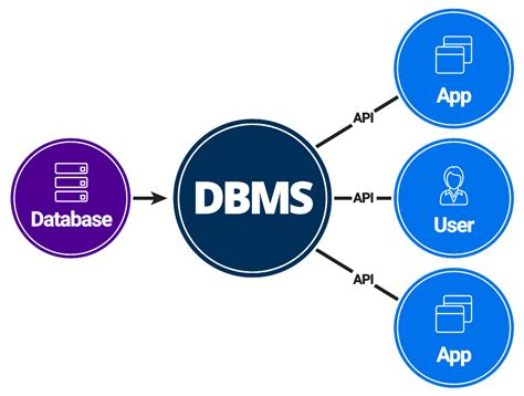
A database management system (DBMS) is a software system that provides an interface for users to interact with databases, allowing them to store, retrieve, update, and manage data efficiently. In bioinformatics, DBMSs are used to store and manage biological data, providing features such as data indexing, query optimization, and transaction management.
The DBMS approach in bioinformatics involves several key aspects:
- Data Modeling: DBMSs use data models to represent the structure of the data stored in the database. In bioinformatics, data models are designed to accommodate the complex relationships between biological entities, such as genes, proteins, and pathways. Common data models used in bioinformatics include relational, object-oriented, and graph-based models.
- Data Storage: DBMSs store biological data in a structured format, such as tables in a relational database. This allows for efficient storage and retrieval of data, as well as the ability to perform complex queries and analyses on the data.
- Data Integration: Bioinformatics databases often contain data from multiple sources, such as genomic sequences, protein structures, and gene expression data. DBMSs allow for the integration of these diverse data types, enabling researchers to analyze relationships and patterns across different datasets.
- Data Querying and Analysis: DBMSs provide a query language, such as SQL (Structured Query Language), that allows users to retrieve and manipulate data stored in the database. In bioinformatics, this enables researchers to perform complex queries and analyses to extract meaningful insights from the data.
- Data Security and Privacy: DBMSs provide mechanisms for ensuring the security and privacy of the data stored in the database. This includes access control mechanisms to restrict who can access the data, as well as encryption and authentication mechanisms to protect the data from unauthorized access.
Overall, the DBMS approach in bioinformatics plays a critical role in managing the vast amounts of biological data generated in research, enabling researchers to store, retrieve, and analyze data efficiently and effectively.
Database system concepts and architecture in bioinformatics
Database systems in bioinformatics follow the same fundamental concepts and architecture as traditional database systems but are tailored to manage biological data effectively. Here are the key concepts and architecture components:
- Data Modeling: Bioinformatics databases often use specialized data models to represent biological entities such as genes, proteins, and sequences. These models may include relational, object-oriented, or graph-based representations, depending on the nature of the data and the requirements of the application.
- Schema: The schema defines the structure of the database, including tables, fields, and relationships between tables. In bioinformatics, the schema is designed to accommodate the complex relationships between biological entities, such as genes, proteins, and pathways.
- Storage: Biological data can be stored in various formats, including raw sequence data, annotations, and metadata. Database systems in bioinformatics must be able to store and retrieve these data types efficiently.
- Indexing: Indexes are used to speed up data retrieval by allowing the database system to quickly locate data based on specified criteria. In bioinformatics, indexing is crucial for efficient retrieval of sequences, genes, and other biological entities.
- Query Language: Bioinformatics databases typically use SQL (Structured Query Language) or specialized query languages to retrieve and manipulate data. These languages allow researchers to perform complex queries and analyses on the data stored in the database.
- Integration: Bioinformatics databases often integrate data from multiple sources, such as genomic sequences, protein structures, and gene expression data. Integration allows researchers to analyze relationships and patterns across different datasets.
- Data Security: Data security is a critical concern in bioinformatics, given the sensitive nature of biological data. Database systems in bioinformatics must implement robust security measures, such as access control and encryption, to protect data from unauthorized access.
- Scalability: As the volume of biological data continues to grow, database systems in bioinformatics must be able to scale to handle large datasets efficiently. This may involve using distributed database systems or cloud-based solutions.
- Data Warehousing: Data warehousing is used to consolidate and integrate data from multiple sources for analysis and reporting. In bioinformatics, data warehousing can be used to create comprehensive repositories of biological data for research purposes.
- Data Mining and Analysis: Database systems in bioinformatics support data mining and analysis techniques to extract useful information from large datasets. This may involve statistical analysis, machine learning, or other computational methods.
Overall, database systems in bioinformatics play a crucial role in managing and analyzing biological data, enabling researchers to make new discoveries and advancements in the field.
Three-schema architecture and data independence
The three-schema architecture is a conceptual framework that separates a database system into three layers: the external schema, the conceptual schema, and the internal schema. This architecture provides a clear separation between different aspects of the database system, which helps in achieving data independence and managing complexity. Here’s an overview of each schema and how they relate to data independence:
- External Schema (View Level): The external schema represents the user’s view of the data. It defines how data is presented and accessed by users or applications. Each external schema corresponds to a specific user or group of users and defines the subset of the conceptual schema that is relevant to them. The external schema provides a level of abstraction that hides the details of the underlying data storage and organization, allowing users to interact with the database in a way that is meaningful to them.
- Data Independence: External schemas provide a degree of data independence known as logical data independence. This means that changes to the conceptual schema (such as adding new tables or modifying existing ones) do not require changes to the external schemas, as long as the external view of the data remains the same. Users can continue to interact with the database using their external schemas without being affected by changes to the underlying database structure.
- Conceptual Schema (Conceptual Level): The conceptual schema represents the logical structure of the entire database, including all the data elements, relationships between them, and constraints. It defines the overall organization of the data and provides a unified view of the database for all users. The conceptual schema is independent of both the external schemas and the internal schema, providing a high-level abstraction of the entire database.
- Data Independence: The conceptual schema provides a higher level of data independence known as conceptual data independence. This means that changes to the internal schema (such as changes to the storage structures or indexing strategies) do not require changes to the conceptual schema, as long as the external schemas are not affected. This allows for greater flexibility in managing the database system, as changes to the physical storage structures can be made without impacting the logical structure of the database.
- Internal Schema (Storage Level): The internal schema represents the physical storage of the data on the underlying hardware. It defines how the data is stored, indexed, and organized to optimize performance and storage efficiency. The internal schema is hidden from users and applications, as it is concerned with the internal workings of the database system.
- Data Independence: The internal schema provides the lowest level of data independence known as physical data independence. This means that changes to the internal schema, such as reorganizing data storage or changing indexing strategies, do not require changes to either the conceptual schema or the external schemas. This allows for the physical storage structures to be modified without impacting the logical or external views of the data.
In summary, the three-schema architecture provides a clear separation between different aspects of the database system, allowing for different levels of data abstraction and independence. This separation helps in managing complexity, improving system flexibility, and providing a clear framework for database design and development.
Centralized and client-server architectures for DBMS in bioinformatics
In bioinformatics, as in other fields, database management systems (DBMS) can be implemented using different architectures. Two common architectures are centralized and client-server. Here’s an overview of each:
- Centralized Architecture:
- Description: In a centralized architecture, the entire DBMS, including the database and the DBMS software, is located on a single server or machine. Users interact with the database through the DBMS software running on that server.
- Advantages:
- Simplicity: Centralized architectures are often simpler to implement and manage, as there is only one server to maintain.
- Performance: In some cases, centralized architectures can offer better performance for certain types of applications, as all data processing occurs on a single server.
- Disadvantages:
- Scalability: Centralized architectures can be challenging to scale as the size of the database or the number of users grows. The single server can become a bottleneck.
- Fault Tolerance: A single point of failure in the centralized server can lead to downtime and data loss.
- Use in Bioinformatics: Centralized architectures may be suitable for smaller bioinformatics projects or labs where the data volume and user load are relatively low.
- Client-Server Architecture:
- Description: In a client-server architecture, the database and the DBMS software are separated from the user interface (client). The database resides on a server, and clients interact with the database through a network, typically using a client application.
- Advantages:
- Scalability: Client-server architectures are more scalable than centralized architectures, as multiple servers can be used to handle increasing data volume and user load.
- Fault Tolerance: Client-server architectures can be designed to be more fault-tolerant, with mechanisms such as replication and load balancing.
- Disadvantages:
- Complexity: Client-server architectures can be more complex to implement and manage, as they require networking infrastructure and coordination between client and server components.
- Performance Overhead: Client-server architectures can introduce additional overhead due to network communication between clients and servers.
- Use in Bioinformatics: Client-server architectures are often preferred for larger bioinformatics projects or organizations where scalability, fault tolerance, and distributed access to the database are important.
In summary, the choice between centralized and client-server architectures for DBMS in bioinformatics depends on factors such as the size and complexity of the project, the expected data volume and user load, and the need for scalability and fault tolerance. Both architectures have their strengths and weaknesses, and the choice should be based on the specific requirements of the bioinformatics application.
Relational Database Design for Bioinformatics
Relational database design using ER-to-Relational mapping
Relational database design involves translating an Entity-Relationship (ER) diagram into a set of relational tables. This process is known as ER-to-Relational mapping. Here’s a step-by-step guide to perform ER-to-Relational mapping:
- Identify Entities: Review the ER diagram to identify the entities (objects) in the system. Each entity becomes a table in the relational database.
- Identify Attributes: For each entity, identify its attributes (properties). Each attribute becomes a column in the corresponding table.
- Identify Keys: Identify the primary key for each table. If the ER diagram specifies a primary key for an entity, it becomes the primary key in the relational table. Otherwise, you may need to choose a suitable candidate key.
- Identify Relationships: Identify the relationships between entities. Relationships are represented using foreign keys in the relational database.
- Convert Weak Entities: If the ER diagram includes weak entities (entities that depend on another entity for their existence), convert them into separate tables with a foreign key referencing the owning entity.
- Convert Many-to-Many Relationships: If the ER diagram includes many-to-many relationships, convert them into separate tables (association tables) with foreign keys referencing the related entities.
- Normalize the Schema (Optional): Normalize the schema to eliminate redundancy and improve data integrity. This may involve splitting tables or creating additional tables to represent complex relationships.
- Review and Refine: Review the relational schema to ensure that it accurately represents the data model and meets the requirements of the system. Refine the schema as necessary to improve performance, maintainability, and usability.
Example: Consider an ER diagram with entities Student and Course, and a many-to-many relationship between them:
- Student (student_id, student_name)
- Course (course_id, course_name)
- Enrollment (student_id, course_id)
In this example, Student and Course are entities that become tables in the relational database. Enrollment is an association table representing the many-to-many relationship between students and courses, with foreign keys referencing the Student and Course tables.
By following these steps, you can map an ER diagram to a relational database schema, ensuring that the database accurately represents the data model and meets the requirements of the system.
Mapping EER model constructs to relations in bioinformatics
In bioinformatics, as in other fields, the Enhanced Entity-Relationship (EER) model can be used to represent complex data relationships and constraints. Mapping EER model constructs to relations in a relational database involves translating the EER model into a set of relational tables. Here’s how you can map some common EER model constructs to relations in bioinformatics:
- Entities: Entities in the EER model represent objects or concepts in the real world, such as genes, proteins, or organisms. Each entity becomes a table in the relational database, with attributes mapped to columns in the table.
For example, a Gene entity in the EER model with attributes gene_id, gene_name, and gene_sequence would be mapped to a Gene table with columns gene_id, gene_name, and gene_sequence.
- Relationships: Relationships in the EER model represent associations between entities. In a relational database, relationships are represented using foreign keys.
For example, a Many-to-Many relationship between Gene and Protein entities in the EER model would be mapped to an Association table in the relational database, linking genes and proteins:
- Gene (gene_id, gene_name, gene_sequence)
- Protein (protein_id, protein_name, protein_sequence)
- GeneProteinAssociation (gene_id, protein_id)
- Inheritance: Inheritance in the EER model represents a hierarchy of entities, where subtypes inherit attributes and relationships from supertypes. In a relational database, inheritance can be implemented using one of several strategies, such as single table inheritance or class table inheritance.
For example, consider a hierarchy of genes in the EER model, with a Gene entity as the supertype and DNAGene and RNAGene entities as subtypes. This could be implemented in a relational database using a single Gene table with a type column to differentiate between DNA and RNA genes:
- Gene (gene_id, gene_name, gene_sequence, type)
- type can be ‘DNA’ or ‘RNA’
- Gene (gene_id, gene_name, gene_sequence, type)
- Aggregation: Aggregation in the EER model represents a relationship where one entity is composed of other entities. In a relational database, aggregation can be represented using foreign keys and separate tables for the aggregated entities.
For example, consider an Aggregation relationship between a Protein entity and a Domain entity, where a protein can be composed of multiple domains. This could be implemented using separate tables for proteins and domains, with a ProteinDomain table to link them:
- Protein (protein_id, protein_name)
- Domain (domain_id, domain_name)
- ProteinDomain (protein_id, domain_id)
By mapping EER model constructs to relations in a relational database, you can effectively represent complex biological data relationships and constraints, facilitating data storage, retrieval, and analysis in bioinformatics applications.
Basic SQL for bioinformatics: data definition, data types, constraints, and basic retrieval queries
SQL (Structured Query Language) is a powerful tool for working with relational databases in bioinformatics. Here’s a basic overview of SQL concepts and queries relevant to bioinformatics:
- Data Definition:
- CREATE TABLE: Used to create a new table in the database.sql
CREATE TABLE Gene (
 gene_id INT PRIMARY KEY,
 gene_name VARCHAR(255),
 chromosome VARCHAR(50),
 start_position INT,
 end_position INT
 );
- CREATE TABLE: Used to create a new table in the database.
- Data Types:
- INT: Integer data type.
- VARCHAR: Variable-length string data type.
- FLOAT: Floating-point number data type.
- DATE: Date data type.
- BOOLEAN: Boolean (true/false) data type.
- Constraints:
- PRIMARY KEY: Ensures that each row in a table is unique and identifies it uniquely.
- FOREIGN KEY: Establishes a relationship between two tables.
- NOT NULL: Ensures that a column cannot have a NULL value.
- UNIQUE: Ensures that all values in a column are unique.
- Basic Retrieval Queries:
- SELECT: Used to retrieve data from one or more tables.sql
SELECT * FROM Gene;
- WHERE: Used to filter rows based on a condition.sql
SELECT * FROM Gene WHERE chromosome = 'X';
- ORDER BY: Used to sort the result set.sql
SELECT * FROM Gene ORDER BY start_position;
- LIMIT: Used to limit the number of rows returned.sql
SELECT * FROM Gene LIMIT 10;
- SELECT: Used to retrieve data from one or more tables.
- Join Operations:
- INNER JOIN: Returns rows when there is at least one match in both tables.sql
SELECT Gene.gene_name, Protein.protein_name
 FROM Gene
 INNER JOIN Protein ON Gene.gene_id = Protein.gene_id;
- LEFT JOIN: Returns all rows from the left table and the matched rows from the right table.sql
SELECT Gene.gene_name, Protein.protein_name
 FROM Gene
 LEFT JOIN Protein ON Gene.gene_id = Protein.gene_id;
- INNER JOIN: Returns rows when there is at least one match in both tables.
- Aggregate Functions:
- COUNT: Returns the number of rows in a table.
- SUM: Returns the sum of values in a column.
- AVG: Returns the average of values in a column.
- MAX: Returns the maximum value in a column.
- MIN: Returns the minimum value in a column.sql
SELECT COUNT(*) FROM Gene;
These are just a few basic SQL concepts and queries commonly used in bioinformatics. SQL provides a rich set of features for managing and querying relational databases, making it a valuable tool for working with biological data.
More SQL for bioinformatics: complex queries, triggers, and views
In bioinformatics, SQL can be used for more than just basic queries. Here are some advanced SQL concepts and queries that can be useful:
- Complex Queries:
- Subqueries: Nested queries that are used within another query. For example, to find genes located on chromosome X:sql
SELECT gene_name
 FROM Gene
 WHERE chromosome = 'X';
- Joins: Combining data from multiple tables. For example, to find genes and their corresponding proteins:sql
SELECT Gene.gene_name, Protein.protein_name
 FROM Gene
 JOIN Protein ON Gene.gene_id = Protein.gene_id;
- Group By: Used with aggregate functions to group rows that have the same values in specified columns. For example, to count the number of genes on each chromosome:sql
SELECT chromosome, COUNT(*) as gene_count
 FROM Gene
 GROUP BY chromosome;
- Subqueries: Nested queries that are used within another query. For example, to find genes located on chromosome X:
- Triggers:
- AFTER INSERT Trigger: Executes after a new row is inserted into a table. For example, to update a log table after inserting a new gene:sql
CREATE TRIGGER after_insert_gene
 AFTER INSERT ON Gene
 FOR EACH ROW
 BEGIN
 INSERT INTO GeneLog (action, gene_id)
 VALUES ('INSERT', NEW.gene_id);
 END;
- BEFORE DELETE Trigger: Executes before a row is deleted from a table. For example, to prevent deletion of genes with associated proteins:sql
CREATE TRIGGER before_delete_gene
 BEFORE DELETE ON Gene
 FOR EACH ROW
 BEGIN
 DECLARE protein_count INT;
 SELECT COUNT(*) INTO protein_count FROM Protein WHERE gene_id = OLD.gene_id;
 IF protein_count > 0 THEN
 SIGNAL SQLSTATE '45000' SET MESSAGE_TEXT = 'Cannot delete gene with associated proteins';
 END IF;
 END;
- AFTER INSERT Trigger: Executes after a new row is inserted into a table. For example, to update a log table after inserting a new gene:
- Views:
- Views are virtual tables that are based on the result of a SQL statement. They can simplify complex queries and provide a layer of abstraction over the underlying tables. For example, to create a view that shows genes and their corresponding proteins:sql
CREATE VIEW GeneProteinView AS
 SELECT Gene.gene_name, Protein.protein_name
 FROM Gene
 JOIN Protein ON Gene.gene_id = Protein.gene_id;
- Views can be queried like tables:sql
SELECT * FROM GeneProteinView;
- Views are virtual tables that are based on the result of a SQL statement. They can simplify complex queries and provide a layer of abstraction over the underlying tables. For example, to create a view that shows genes and their corresponding proteins:
These advanced SQL concepts and queries can help in performing complex data analysis and management tasks in bioinformatics, making SQL a valuable tool for working with biological data.
Relational algebra operations for bioinformatics: select, project, join, and division
Relational algebra is a formal system for manipulating relational data, which is the foundation of SQL and relational databases. Here are some key relational algebra operations and how they can be applied in bioinformatics:
- Select (σ): Selects tuples from a relation that satisfy a given condition. In bioinformatics, this can be used to filter rows based on specific criteria. For example, selecting genes on chromosome X:scss
σ(chromosome='X')(Gene)
- Project (π): Projects a subset of columns from a relation. In bioinformatics, this can be used to select specific attributes of interest. For example, projecting gene names and sequences:scss
π(gene_name, gene_sequence)(Gene)
- Join (⨝): Combines tuples from two relations based on a common attribute. In bioinformatics, this can be used to merge data from different tables. For example, joining genes with their corresponding proteins:
Gene ⨝ Protein
- Division (÷): Divides one relation by another to find tuples in the first relation that are related to all tuples in the second relation. This operation is less commonly used in practice but can be useful in certain scenarios. For example, finding genes that are associated with all specified proteins:
Gene ÷ {Protein1, Protein2, ...}
These relational algebra operations provide a formal and mathematical way to manipulate relational data, which can be applied in bioinformatics for data analysis and querying in relational database systems.
Functional Dependencies and Normalization for Bioinformatics
Functional dependencies and normalization for bioinformatics
Functional dependencies and normalization are important concepts in database design, including in bioinformatics, as they help ensure data integrity and efficiency. Here’s an overview of these concepts:
- Functional Dependencies (FDs):
- Definition: A functional dependency is a relationship between two sets of attributes in a relation, where one set of attributes uniquely determines the other set.
- Example: In a gene table, if gene_id uniquely determines gene_name, then we can say that gene_name is functionally dependent on gene_id (gene_id → gene_name).
- Use in Bioinformatics: Understanding functional dependencies helps in designing tables that minimize redundancy and maintain data integrity. For example, ensuring that each gene_id corresponds to a unique gene_name prevents duplicate gene entries.
- Normalization:
- Definition: Normalization is the process of organizing data in a database to reduce redundancy and dependency by breaking up large tables into smaller, related tables.
- Normal Forms: There are several normal forms (NFs), each with its own set of rules for ensuring data integrity and efficiency. The most common normal forms are:
- First Normal Form (1NF): Ensures that each attribute in a table contains only atomic values and that there are no repeating groups or arrays.
- Second Normal Form (2NF): Ensures that each non-key attribute is fully functionally dependent on the primary key.
- Third Normal Form (3NF): Ensures that each non-key attribute is non-transitively dependent on the primary key.
- Example: Suppose we have a table with gene_id, gene_name, chromosome, and start_position. If gene_name is functionally dependent on gene_id, we can normalize the table by creating a separate table for gene_id and gene_name, eliminating redundancy.
Normalization in bioinformatics databases helps in organizing complex biological data efficiently, reducing data redundancy, and ensuring data integrity. It also makes the database easier to maintain and query.
Informal design guidelines for relation schemas in bioinformatics
Designing relation schemas in bioinformatics involves considering the specific characteristics of biological data and the requirements of the database system. Here are some informal design guidelines for relation schemas in bioinformatics:
- Use Meaningful Names: Use descriptive and meaningful names for tables and attributes to make the schema easy to understand. For example, use “Gene” instead of “Table1” and “gene_name” instead of “col1”.
- Normalize the Schema: Normalize the schema to reduce redundancy and dependency. Use the principles of normalization (e.g., 1NF, 2NF, 3NF) to ensure that each table represents a single entity and that there are no repeating groups or arrays.
- Capture Relationships: Capture relationships between entities using foreign keys. For example, if a gene is associated with a protein, use a foreign key in the protein table that references the gene table.
- Consider Data Integrity: Enforce data integrity constraints to ensure the accuracy and consistency of data. Use primary keys, foreign keys, and other constraints to prevent invalid data from being inserted or updated.
- Use Appropriate Data Types: Use appropriate data types for attributes based on the nature of the data. For example, use VARCHAR for text data, INT for integer data, and DATE for date data.
- Avoid Over-Normalization: While normalization is important, avoid over-normalizing the schema, which can lead to complex join operations and performance issues. Strike a balance between normalization and performance.
- Consider Performance: Design the schema with performance in mind. Consider the types of queries that will be performed on the database and design the schema to optimize these queries.
- Document the Schema: Document the schema design, including the rationale behind the design decisions, to make it easier for others to understand and maintain the database.
By following these guidelines, you can design relation schemas in bioinformatics that are efficient, easy to understand, and maintainable, facilitating the management and analysis of biological data.
Normal forms based on primary keys for bioinformatics
In bioinformatics, as in other fields, normal forms are used to ensure that a database schema is well-structured, free of redundancy, and maintains data integrity. Normal forms are based on functional dependencies, which describe the relationships between attributes in a relation. Here’s a brief overview of normal forms based on primary keys:
- First Normal Form (1NF):
- A relation is in 1NF if it does not contain repeating groups or arrays, and each attribute contains only atomic values.
- Example: If a gene table has a column for gene_name that contains multiple values separated by commas (e.g., “gene1, gene2”), it violates 1NF. To normalize, you would create a separate table for gene names and link it to the gene table using a foreign key.
- Second Normal Form (2NF):
- A relation is in 2NF if it is in 1NF and every non-prime attribute (i.e., attributes not part of the primary key) is fully functionally dependent on the primary key.
- Example: If a gene table has attributes gene_id, chromosome, and start_position, and gene_name is functionally dependent on gene_id, then it is in 2NF.
- Third Normal Form (3NF):
- A relation is in 3NF if it is in 2NF and every non-prime attribute is non-transitively dependent on the primary key.
- Example: If a gene table has attributes gene_id, chromosome, start_position, and species_name, where species_name is dependent on chromosome, which is not a key attribute, it violates 3NF. To normalize, you would move species_name to a separate table.
In bioinformatics, normalizing the database schema helps in organizing complex biological data efficiently, reducing redundancy, and ensuring data integrity. It also makes the database easier to maintain and query.
Query processing and optimization in bioinformatics
Query processing and optimization in bioinformatics databases are crucial for efficient data retrieval and analysis, especially when dealing with large datasets. Here are some key aspects of query processing and optimization in bioinformatics:
- Indexing: Indexes are used to speed up data retrieval by creating pointers to data based on specific columns. In bioinformatics, indexing is important for quickly accessing genetic sequences, gene names, or other commonly queried attributes.
- Query Optimization: Query optimization involves choosing the most efficient way to execute a query by considering factors such as indexes, join methods, and data distribution. In bioinformatics, optimizing queries can significantly improve the performance of data analysis tasks.
- Parallel Processing: Parallel processing involves splitting a query into smaller tasks that can be executed simultaneously on multiple processors or nodes. In bioinformatics, parallel processing can be used to speed up tasks such as sequence alignment or genome assembly.
- Data Partitioning: Data partitioning involves dividing a large dataset into smaller chunks that can be processed independently. In bioinformatics, data partitioning can be used to distribute genomic data across multiple nodes in a cluster for parallel processing.
- Caching: Caching involves storing the results of frequently executed queries in memory for faster access. In bioinformatics, caching can be used to store intermediate results of data analysis tasks to avoid recomputation.
- Query Language Optimization: Optimizing the query language used to interact with the database can also improve performance. For example, using efficient SQL queries or optimizing the use of BioSQL or other bioinformatics-specific query languages.
- Hardware Optimization: Hardware optimization involves using specialized hardware, such as GPUs or FPGAs, to accelerate certain types of bioinformatics computations, such as sequence alignment or protein structure prediction.
By employing these techniques, bioinformatics researchers and database administrators can improve the performance of data retrieval and analysis, enabling faster and more efficient processing of biological data.
Transaction Processing and Concurrency Control for Bioinformatics
Introduction to transaction processing in bioinformatics
Transaction processing in bioinformatics involves managing and processing database transactions related to biological data. A transaction is a logical unit of work that consists of one or more database operations, such as insertions, deletions, or updates, which must be executed atomically and consistently. Here’s an introduction to transaction processing in bioinformatics:
- ACID Properties: Transactions in bioinformatics databases are typically expected to adhere to the ACID properties:
- Atomicity: Transactions are all-or-nothing. Either all operations in a transaction are completed successfully, or none of them are.
- Consistency: Transactions bring the database from one consistent state to another consistent state.
- Isolation: Transactions are isolated from each other, meaning that the effects of one transaction are not visible to other transactions until it is completed.
- Durability: Once a transaction is committed, its effects are permanent and survive system failures.
- Database Locking: Transaction processing in bioinformatics often involves the use of database locking mechanisms to ensure that transactions are executed serially or in a specific order to maintain data integrity. Locks can be applied at various levels, such as row-level, table-level, or database-level, depending on the granularity required.
- Concurrency Control: Concurrency control mechanisms are used to manage simultaneous access to data by multiple transactions. Techniques such as locking, timestamping, and optimistic concurrency control are used to ensure that transactions do not interfere with each other.
- Transaction Management: Transaction management involves coordinating the execution of transactions, including starting, committing, and rolling back transactions. In bioinformatics, transaction management ensures that data is processed accurately and consistently.
- Data Integrity: Ensuring data integrity is crucial in bioinformatics transactions. This includes enforcing constraints, such as primary key constraints and foreign key constraints, to maintain data consistency and accuracy.
- Transaction Logging: Transaction logging is used to record the changes made by transactions to the database. This information can be used for recovery purposes in case of system failures or errors.
Overall, transaction processing in bioinformatics plays a critical role in managing and processing biological data, ensuring data integrity, consistency, and reliability in database operations.
Desirable properties of transactions for bioinformatics
In bioinformatics, transactions play a crucial role in managing and processing biological data. The desirable properties of transactions in bioinformatics are similar to those in other fields and include:
- Atomicity: Transactions should be atomic, meaning that either all operations within a transaction are completed successfully, or none of them are. This property ensures that the database remains in a consistent state, especially when dealing with complex biological data.
- Consistency: Transactions should maintain the consistency of the database. This means that transactions should bring the database from one consistent state to another consistent state, adhering to all integrity constraints and business rules.
- Isolation: Transactions should be isolated from each other, meaning that the effects of one transaction should not be visible to other transactions until it is completed. This property ensures that transactions can be executed concurrently without interfering with each other.
- Durability: Once a transaction is committed, its effects should be permanent and survive system failures. This property ensures that data is not lost due to system crashes or other failures.
- Concurrency Control: Transactions should be able to execute concurrently while maintaining the consistency and integrity of the database. Concurrency control mechanisms, such as locking and timestamping, are used to ensure that transactions do not interfere with each other.
- Data Integrity: Transactions should ensure the integrity of the data in the database. This includes enforcing constraints, such as primary key constraints and foreign key constraints, to maintain data consistency and accuracy.
- Efficiency: Transactions should be executed efficiently to minimize the use of system resources and ensure optimal performance, especially when dealing with large volumes of biological data.
By ensuring these properties, transactions in bioinformatics can effectively manage and process biological data, maintaining data integrity, consistency, and reliability in database operations.
Concurrency control techniques for bioinformatics: two-phase locking, timestamp ordering
Concurrency control is essential in bioinformatics to manage simultaneous access to data by multiple transactions while maintaining data consistency and integrity. Two common concurrency control techniques are two-phase locking and timestamp ordering.
- Two-Phase Locking (2PL):
- Description: Two-phase locking is a concurrency control technique that ensures serializability of transactions by acquiring all the locks it needs before starting execution (the growing phase) and releasing all locks when it completes (the shrinking phase).
- Implementation: In bioinformatics, 2PL can be used to manage access to genetic data, ensuring that only one transaction can modify a gene sequence at a time to prevent conflicts and maintain data consistency.
- Advantages: Provides a simple and effective way to control concurrency and ensure transaction isolation.
- Disadvantages: Can lead to lock contention and reduced concurrency if transactions hold locks for long periods, impacting performance.
- Timestamp Ordering:
- Description: Timestamp ordering is a concurrency control technique that assigns a unique timestamp to each transaction based on its start time. Transactions are ordered based on their timestamps, and conflicts are resolved by comparing timestamps.
- Implementation: In bioinformatics, timestamp ordering can be used to manage access to genomic data, ensuring that transactions are executed in a serializable order based on their timestamps.
- Advantages: Allows for more concurrency compared to 2PL, as transactions only need to be ordered based on their timestamps rather than acquiring and releasing locks.
- Disadvantages: May lead to the need for frequent rollbacks and re-executions of transactions to maintain consistency, especially in cases of conflicting transactions.
Both two-phase locking and timestamp ordering are important concurrency control techniques in bioinformatics, each with its own advantages and disadvantages. The choice of technique depends on the specific requirements of the application and the nature of the data being processed.
Database recovery techniques for bioinformatics: ARIES recovery algorithm
The ARIES (Algorithm for Recovery and Isolation Exploiting Semantics) recovery algorithm is a database recovery technique that provides high-performance recovery and concurrency control. It is well-suited for bioinformatics databases where data integrity and recovery from failures are critical. Here’s an overview of the ARIES recovery algorithm:
- Logging: ARIES uses a write-ahead logging (WAL) protocol, where all changes to the database are first recorded in a log before being applied to the actual database. This ensures that changes are durable and can be replayed in case of a failure.
- Transaction Table (TT): ARIES maintains a transaction table (TT) to keep track of active and committed transactions. The TT also stores information about the last log record for each transaction, known as the transaction’s lastLSN.
- Dirty Page Table (DPT): ARIES maintains a dirty page table (DPT) to keep track of all modified pages in the buffer pool that have not yet been written to disk. This allows ARIES to efficiently redo or undo changes during recovery.
- Analysis Phase: During recovery, ARIES first performs an analysis phase where it scans the log from the most recent checkpoint to the end to identify all transactions that were active at the time of the crash and all dirty pages in the buffer pool.
- Redo Phase: After the analysis phase, ARIES performs a redo phase where it re-applies all changes recorded in the log that were not yet written to disk. This ensures that all committed changes are restored to the database.
- Undo Phase: Finally, ARIES performs an undo phase where it rolls back all changes made by transactions that were active at the time of the crash but had not yet committed. This ensures that the database is restored to a consistent state.
Overall, the ARIES recovery algorithm provides efficient and reliable recovery from failures in bioinformatics databases, ensuring data integrity and consistency. Its use of logging, transaction tables, and dirty page tables makes it well-suited for high-performance databases where fast recovery and concurrency control are essential.
Indexing Structures and NoSQL Databases for Bioinformatics
Indexing structures for files and physical database design in bioinformatics
In bioinformatics, as in other fields, indexing structures play a crucial role in file and database design to optimize data retrieval and query performance. Here are some common indexing structures used in bioinformatics:
- B-tree and B+-tree: B-trees and B+-trees are widely used indexing structures in bioinformatics for organizing and accessing data efficiently. They are particularly useful for indexing genomic data, such as DNA sequences, gene sequences, or protein sequences.
- Hash Indexes: Hash indexes can be used to quickly locate data based on a hash value. They are often used in bioinformatics for indexing large datasets, such as genomic sequences or protein sequences, where fast access to specific data points is essential.
- Inverted Indexes: Inverted indexes are commonly used in bioinformatics for full-text search operations. They are useful for indexing text data, such as genetic sequences or biomedical literature, allowing for fast retrieval of relevant information based on keywords or patterns.
- Suffix Trees and Suffix Arrays: Suffix trees and suffix arrays are indexing structures used for efficient substring search in bioinformatics. They are commonly used for indexing DNA sequences, protein sequences, or other biological sequences for pattern matching and similarity search.
- Spatial Indexes: Spatial indexes, such as R-trees, are used in bioinformatics for indexing spatial data, such as the three-dimensional structure of proteins or the spatial distribution of genes on a chromosome. They enable efficient retrieval of spatially related data points.
- Bitmap Indexes: Bitmap indexes are useful for indexing categorical data with a limited number of distinct values. In bioinformatics, bitmap indexes can be used for indexing gene expression data, where each gene can be associated with multiple conditions or treatments.
In addition to choosing the appropriate indexing structure, it is also important to consider the physical database design, including storage layout, data partitioning, and replication strategies, to optimize query performance and data access in bioinformatics applications.
Single level and multi-level indexing for bioinformatics
In bioinformatics, indexing plays a crucial role in efficiently storing and retrieving large volumes of biological data. Two common types of indexing used in bioinformatics are single-level indexing and multi-level indexing.
- Single-Level Indexing:
- Description: Single-level indexing involves creating an index structure that directly maps keys to their corresponding data blocks or records.
- Implementation: In bioinformatics, single-level indexing can be used to index genetic sequences, gene names, or protein identifiers, allowing for fast retrieval of specific sequences or genes.
- Advantages: Simple and straightforward to implement, suitable for smaller datasets or when the index keys have a one-to-one mapping with data blocks.
- Disadvantages: May not scale well for large datasets, as the entire index needs to be searched linearly to find a specific key.
- Multi-Level Indexing:
- Description: Multi-level indexing involves creating a hierarchical index structure with multiple levels, where each level points to a lower level of the index.
- Implementation: In bioinformatics, multi-level indexing can be used to index large datasets, such as genomic sequences or protein structures, by dividing the index into multiple levels based on sequence similarity or other criteria.
- Advantages: Scales well for large datasets, as it reduces the number of comparisons needed to find a specific key.
- Disadvantages: More complex to implement compared to single-level indexing, may require additional storage space for the index structure.
In bioinformatics, the choice between single-level and multi-level indexing depends on the size and complexity of the dataset, as well as the specific requirements of the application. Single-level indexing may be more suitable for smaller datasets or when the index keys have a simple structure, while multi-level indexing is more appropriate for larger datasets with complex relationships between keys.
Introduction to NoSQL databases for bioinformatics
NoSQL (Not Only SQL) databases are a category of database management systems that are characterized by their non-relational data models. They are designed to handle large volumes of data, provide high availability, and scale horizontally across multiple servers. In bioinformatics, NoSQL databases offer several advantages for managing and analyzing biological data. Here’s an introduction to NoSQL databases for bioinformatics:
- Types of NoSQL Databases:
- Document Store: Stores data in flexible, JSON-like documents. Examples include MongoDB and CouchDB.
- Key-Value Store: Stores data as key-value pairs. Examples include Redis and DynamoDB.
- Column-Family Store: Stores data in columns rather than rows. Examples include Cassandra and HBase.
- Graph Database: Stores data in nodes and edges to represent relationships. Examples include Neo4j and Amazon Neptune.
- Advantages of NoSQL Databases for Bioinformatics:
- Schema-less Design: NoSQL databases do not require a fixed schema, making it easier to store and query diverse types of biological data.
- Horizontal Scalability: NoSQL databases can scale horizontally by adding more servers, making them suitable for handling large-scale bioinformatics datasets.
- High Performance: NoSQL databases are optimized for performance, allowing for faster data retrieval and analysis.
- Flexible Data Models: NoSQL databases support flexible data models, making it easier to store complex biological data structures, such as genomic sequences or protein structures.
- Use Cases in Bioinformatics:
- Genomic Data Storage: NoSQL databases can store large genomic datasets, such as DNA sequences, gene annotations, and variation data.
- Biological Network Analysis: Graph databases are well-suited for storing and analyzing biological networks, such as protein-protein interaction networks or metabolic pathways.
- Text Mining and Literature Analysis: NoSQL databases can be used to store and query biomedical literature, enabling text mining and literature analysis for bioinformatics research.
- Challenges and Considerations:
- Data Consistency: NoSQL databases may sacrifice some level of data consistency for scalability and performance, which may be a concern for certain bioinformatics applications.
- Query Language: NoSQL databases often use different query languages than traditional SQL databases, which may require bioinformaticians to learn new skills.
In conclusion, NoSQL databases offer several advantages for bioinformatics, including scalability, performance, and flexibility, making them a valuable tool for managing and analyzing large and complex biological datasets.
Document-based NoSQL systems and MongoDB for bioinformatics applications
Document-based NoSQL databases, such as MongoDB, are well-suited for bioinformatics applications due to their flexibility, scalability, and ability to handle complex and varied data structures. MongoDB, in particular, is a popular choice in bioinformatics for its ease of use, powerful querying capabilities, and support for high-throughput data processing. Here’s how MongoDB can be used in bioinformatics applications:
- Flexible Data Model: MongoDB stores data in flexible, JSON-like documents, which makes it ideal for storing diverse biological data, such as genomic sequences, gene annotations, and experimental results. The schema-less design allows for easy storage and retrieval of complex data structures.
- Scalability: MongoDB is designed to scale horizontally across multiple servers, making it suitable for handling large-scale bioinformatics datasets. It can efficiently manage growing volumes of data without sacrificing performance.
- High Performance: MongoDB is optimized for performance, with support for indexing, aggregation, and ad-hoc queries. This makes it well-suited for real-time analysis of biological data, such as sequence alignments or variant calling.
- Geospatial Queries: MongoDB’s support for geospatial queries can be useful in bioinformatics for analyzing spatial data, such as the distribution of genes on a chromosome or the location of genetic markers.
- Data Replication and High Availability: MongoDB supports data replication and automatic failover, ensuring high availability and data durability. This is important in bioinformatics where data integrity and availability are critical.
- Integration with Bioinformatics Tools: MongoDB can be easily integrated with other bioinformatics tools and libraries, such as Biopython or Bioconductor, allowing for seamless data exchange and analysis.
Overall, MongoDB is a powerful and versatile NoSQL database that offers many benefits for bioinformatics applications. Its flexible data model, scalability, and performance make it a valuable tool for managing and analyzing biological data.
Laboratory Experiments
Designing conceptual database schemas using ER modeling tools for bioinformatics
Designing conceptual database schemas for bioinformatics involves using Entity-Relationship (ER) modeling tools to create a graphical representation of the database schema. ER modeling helps to visualize the entities (objects or concepts), attributes (properties of entities), and relationships (associations between entities) in the database. Here’s a general approach to designing conceptual database schemas using ER modeling tools for bioinformatics:
- Identify Entities: Identify the main entities in your bioinformatics database. These could include biological entities such as genes, proteins, sequences, or experimental data.
- Define Attributes: For each entity, define the attributes that describe it. Attributes could include properties such as gene name, sequence data, or experimental conditions.
- Identify Relationships: Identify the relationships between entities. For example, a gene may be associated with one or more proteins, or a sequence may be part of a specific genome.
- Create ER Diagram: Use an ER modeling tool to create a diagram that visually represents the entities, attributes, and relationships in your database. Entities are represented as boxes, attributes as ovals, and relationships as lines connecting entities.
- Refine the Schema: Refine the schema based on feedback and requirements. This may involve adding or removing entities, attributes, or relationships to better represent the data and its relationships.
- Document the Schema: Document the schema by providing descriptions of entities, attributes, and relationships. This documentation helps others understand the structure and purpose of the database.
- Validate the Schema: Validate the schema to ensure that it accurately represents the data and meets the requirements of the bioinformatics application.
By following these steps, you can design a conceptual database schema using ER modeling tools that effectively represents the data and relationships in your bioinformatics database.
Developing relational database schemas for bioinformatics using SQL DDL constructs
Developing a relational database schema for bioinformatics involves using SQL Data Definition Language (DDL) constructs to define tables, columns, keys, and constraints. Here’s a general approach to developing a relational database schema for bioinformatics using SQL DDL:
- Identify Entities: Identify the main entities in your bioinformatics application. These could include genes, proteins, sequences, experiments, and other relevant entities.
- Define Tables: For each entity, create a table in the database. Use the CREATE TABLE statement to define the table structure, including column names, data types, and constraints.sql
CREATE TABLE genes (
 gene_id INT PRIMARY KEY,
 gene_name VARCHAR(255),
 chromosome VARCHAR(255),
 start_position INT,
 end_position INT
 );
- Define Relationships: Identify and define relationships between entities. Use foreign keys to establish relationships between tables.sql
CREATE TABLE proteins (
 protein_id INT PRIMARY KEY,
 gene_id INT,
 FOREIGN KEY (gene_id) REFERENCES genes(gene_id)
 );
- Define Constraints: Define constraints to enforce data integrity rules, such as uniqueness and referential integrity.sql
CREATE TABLE sequences (
 sequence_id INT PRIMARY KEY,
 gene_id INT,
 sequence_data TEXT,
 FOREIGN KEY (gene_id) REFERENCES genes(gene_id)
 );
- Indexing: Consider adding indexes to columns that are frequently used in queries to improve query performance.sql
CREATE INDEX idx_gene_name ON genes(gene_name);
- Normalization: Normalize the database schema to reduce redundancy and improve data integrity. This may involve splitting tables into smaller tables and using foreign keys to link them.
- Review and Refine: Review the schema to ensure that it accurately represents the data model and meets the requirements of the bioinformatics application. Refine the schema as needed based on feedback and requirements.
- Document the Schema: Document the schema by providing descriptions of tables, columns, relationships, and constraints. This documentation helps others understand the database structure and use it effectively.
By following these steps and using SQL DDL constructs, you can develop a relational database schema for bioinformatics that effectively represents the data model and meets the requirements of your application.
Specifying various DML commands in SQL on relational databases for bioinformatics
In bioinformatics, SQL (Structured Query Language) is used to manipulate data in relational databases. Here are some common Data Manipulation Language (DML) commands in SQL that are relevant to bioinformatics:
- SELECT: The SELECT statement is used to retrieve data from one or more tables. It can be used to retrieve specific columns, filter rows based on conditions, and perform calculations on data.sql
SELECT gene_name, chromosome
 FROM genes
 WHERE chromosome = 'X';
- INSERT: The INSERT statement is used to insert new rows of data into a table.sql
INSERT INTO genes (gene_name, chromosome, start_position, end_position)
 VALUES ('ABC', 'X', 1000, 2000);
- UPDATE: The UPDATE statement is used to modify existing data in a table.sql
UPDATE genes
 SET start_position = 1500
 WHERE gene_name = 'ABC';
- DELETE: The DELETE statement is used to remove rows from a table based on specified criteria.sql
DELETE FROM genes
 WHERE gene_name = 'ABC';
- MERGE (UPSERT): The MERGE statement is used to perform an “upsert” operation, which inserts a new row if it does not exist or updates an existing row if it does.sql
MERGE INTO genes g
 USING (SELECT 'ABC' AS gene_name, 'X' AS chromosome, 1000 AS start_position, 2000 AS end_position) AS new_gene
 ON g.gene_name = new_gene.gene_name
 WHEN MATCHED THEN
 UPDATE SET g.chromosome = new_gene.chromosome, g.start_position = new_gene.start_position, g.end_position = new_gene.end_position
 WHEN NOT MATCHED THEN
 INSERT (gene_name, chromosome, start_position, end_position) VALUES (new_gene.gene_name, new_gene.chromosome, new_gene.start_position, new_gene.end_position);
- Transaction Control Statements: SQL provides commands to control transactions, such as COMMIT to save changes, ROLLBACK to undo changes, and SAVEPOINT to set a savepoint within a transaction.sql
BEGIN TRANSACTION;
 -- SQL statements
 COMMIT;
These are just a few examples of DML commands in SQL that are commonly used in bioinformatics. SQL is a powerful language that allows for complex data manipulation operations, making it a valuable tool for managing and analyzing biological data.
Development of relational database schemas by specifying different types of constraints for bioinformatics
In bioinformatics, developing a relational database schema involves specifying various types of constraints to ensure data integrity and consistency. Here are some common types of constraints used in relational databases for bioinformatics:
- Primary Key Constraint: Ensures that each row in a table is uniquely identified by a primary key. This constraint prevents duplicate records and allows for efficient data retrieval.sql
CREATE TABLE genes (
 gene_id INT PRIMARY KEY,
 gene_name VARCHAR(255),
 chromosome VARCHAR(255),
 start_position INT,
 end_position INT
 );
- Foreign Key Constraint: Ensures that the values in a column (or set of columns) in one table match the values in a column (or set of columns) in another table. This constraint is used to enforce referential integrity between related tables.sql
CREATE TABLE proteins (
 protein_id INT PRIMARY KEY,
 gene_id INT,
 FOREIGN KEY (gene_id) REFERENCES genes(gene_id)
 );
- Unique Constraint: Ensures that the values in a column (or set of columns) are unique across all rows in the table. This constraint is used to enforce uniqueness of data.sql
CREATE TABLE sequences (
 sequence_id INT PRIMARY KEY,
 gene_id INT,
 sequence_data TEXT,
 UNIQUE (gene_id)
 );
- Check Constraint: Ensures that the values in a column meet a specific condition. This constraint is used to enforce data integrity rules.sql
CREATE TABLE experiments (
 experiment_id INT PRIMARY KEY,
 experiment_date DATE,
 status VARCHAR(255),
 CHECK (status IN ('ongoing', 'completed', 'cancelled'))
 );
- Not Null Constraint: Ensures that a column does not contain null values. This constraint is used to enforce mandatory data entry.sql
CREATE TABLE samples (
 sample_id INT PRIMARY KEY,
 sample_name VARCHAR(255) NOT NULL,
 collection_date DATE,
 organism VARCHAR(255)
 );
- Default Constraint: Specifies a default value for a column if no value is provided. This constraint is used to ensure that a column always contains a value.sql
CREATE TABLE patients (
 patient_id INT PRIMARY KEY,
 patient_name VARCHAR(255),
 gender VARCHAR(255) DEFAULT 'Unknown'
 );
These are some common types of constraints used in relational database schemas for bioinformatics. By specifying these constraints, you can ensure that your database maintains data integrity and consistency, which is crucial for accurate and reliable data analysis in bioinformatics.
Specifying queries using relational database operators and string matching constructs in SQL for bioinformatics
In bioinformatics, SQL queries are commonly used to retrieve, filter, and analyze data stored in relational databases. Here are some examples of SQL queries that use relational database operators and string matching constructs:
- SELECT Statement: The SELECT statement is used to retrieve data from one or more tables.sql
SELECT * FROM genes;
- WHERE Clause: The WHERE clause is used to filter rows based on a specified condition.sql
SELECT * FROM genes WHERE chromosome = 'X';
- LIKE Operator: The LIKE operator is used for pattern matching in string columns.sql
SELECT * FROM genes WHERE gene_name LIKE 'ABC%';
- IN Operator: The IN operator is used to specify multiple values in a WHERE clause.sql
SELECT * FROM genes WHERE chromosome IN ('X', 'Y');
- BETWEEN Operator: The BETWEEN operator is used to specify a range of values in a WHERE clause.sql
SELECT * FROM genes WHERE start_position BETWEEN 1000 AND 2000;
- ORDER BY Clause: The ORDER BY clause is used to sort the result set based on one or more columns.sql
SELECT * FROM genes ORDER BY gene_name ASC;
- GROUP BY Clause: The GROUP BY clause is used to group rows that have the same values in specified columns.sql
SELECT chromosome, COUNT(*) AS gene_count FROM genes GROUP BY chromosome;
- JOIN Clause: The JOIN clause is used to combine rows from two or more tables based on a related column between them.sql
SELECT genes.gene_name, proteins.protein_name
 FROM genes
 JOIN proteins ON genes.gene_id = proteins.gene_id;
- Aggregate Functions: Aggregate functions like COUNT, SUM, AVG, MIN, and MAX can be used to perform calculations on groups of rows.sql
SELECT chromosome, COUNT(*) AS gene_count
 FROM genes
 GROUP BY chromosome;
- Subqueries: Subqueries can be used to nest one query inside another query.sql
SELECT * FROM genes WHERE gene_id IN (SELECT gene_id FROM proteins);
These are just a few examples of SQL queries that use relational database operators and string matching constructs in bioinformatics. SQL is a powerful language that can be used to perform complex data retrieval and analysis tasks on relational databases.
Expressing queries using aggregate functions of SQL on relational databases for bioinformatics
In bioinformatics, aggregate functions in SQL are often used to perform calculations on groups of rows or to summarize data. Here are some examples of SQL queries that use aggregate functions for bioinformatics:
- COUNT Function: Counts the number of rows in a table or the number of rows that meet a specific condition.sql
SELECT COUNT(*) FROM genes;
- SUM Function: Calculates the sum of values in a column.sql
SELECT SUM(expression) FROM table_name;
- AVG Function: Calculates the average value of a column.sql
SELECT AVG(expression) FROM table_name;
- MIN Function: Finds the minimum value in a column.sql
SELECT MIN(expression) FROM table_name;
- MAX Function: Finds the maximum value in a column.sql
SELECT MAX(expression) FROM table_name;
- GROUP BY Clause with Aggregate Functions: Used to group rows that have the same values in specified columns and perform aggregate functions on each group.sql
SELECT chromosome, COUNT(*) AS gene_count
FROM genes
GROUP BY chromosome;
- HAVING Clause: Used in combination with the GROUP BY clause to filter groups based on a specified condition.sql
SELECT chromosome, COUNT(*) AS gene_count
 FROM genes
 GROUP BY chromosome
 HAVING COUNT(*) > 100;
- Nested Aggregate Functions: Aggregate functions can be nested to perform calculations on the results of other aggregate functions.sql
SELECT AVG(gene_count) AS avg_gene_count
 FROM (
 SELECT chromosome, COUNT(*) AS gene_count
 FROM genes
 GROUP BY chromosome
 ) AS gene_counts;
- DISTINCT Keyword: Used to eliminate duplicate rows from the result set when using aggregate functions.sql
SELECT COUNT(DISTINCT chromosome) AS distinct_chromosomes
 FROM genes;
These are some examples of how aggregate functions can be used in SQL queries for bioinformatics to perform calculations and summarize data in relational databases.
Queries on relational databases using GROUP BY, HAVING, and ORDER BY clauses in SQL for bioinformatics
In bioinformatics, SQL queries often involve grouping, filtering, and ordering data to extract meaningful information from relational databases. Here are examples of SQL queries that use the GROUP BY, HAVING, and ORDER BY clauses for bioinformatics:
- GROUP BY Clause: Groups rows that have the same values in specified columns and allows for aggregation functions to be applied to each group.sql
SELECT chromosome, COUNT(*) AS gene_count
 FROM genes
 GROUP BY chromosome;
- HAVING Clause: Filters groups based on a specified condition. It is used in combination with the GROUP BY clause.sql
SELECT chromosome, COUNT(*) AS gene_count
 FROM genes
 GROUP BY chromosome
 HAVING COUNT(*) > 100;
- ORDER BY Clause: Sorts the result set based on one or more columns. By default, sorting is done in ascending order (ASC), but you can specify descending order (DESC) as well.sql
SELECT gene_name, start_position, end_position
 FROM genes
 ORDER BY start_position DESC;
- Combining GROUP BY, HAVING, and ORDER BY: You can combine these clauses to perform more complex queries. For example, to find the chromosome with the highest number of genes:sql
SELECT chromosome, COUNT(*) AS gene_count
 FROM genes
 GROUP BY chromosome
 HAVING COUNT(*) = (
 SELECT MAX(gene_count)
 FROM (
 SELECT COUNT(*) AS gene_count
 FROM genes
 GROUP BY chromosome
 ) AS counts
 )
 ORDER BY chromosome;
- Using Aggregate Functions with GROUP BY: You can use aggregate functions with the GROUP BY clause to calculate summary statistics for each group.sql
SELECT chromosome, MIN(start_position) AS min_start, MAX(end_position) AS max_end
 FROM genes
 GROUP BY chromosome
 ORDER BY chromosome;
These examples demonstrate how the GROUP BY, HAVING, and ORDER BY clauses can be used in SQL queries for bioinformatics to group, filter, and sort data in relational databases.
Design and development of company database and expressing nested queries using SQL for bioinformatics
Designing and developing a company database for bioinformatics involves creating tables to store information about employees, projects, clients, and other relevant entities. Here’s a basic example of how you might design such a database, along with some examples of nested queries using SQL:
- Database Design:
- Employees Table: Contains information about company employees.sql
CREATE TABLE employees (
 employee_id INT PRIMARY KEY,
 employee_name VARCHAR(255),
 department VARCHAR(255),
 hire_date DATE
 );
- Projects Table: Contains information about projects undertaken by the company.sql
CREATE TABLE projects (
 project_id INT PRIMARY KEY,
 project_name VARCHAR(255),
 start_date DATE,
 end_date DATE,
 lead_employee_id INT,
 FOREIGN KEY (lead_employee_id) REFERENCES employees(employee_id)
 );
- Clients Table: Contains information about clients.sql
CREATE TABLE clients (
 client_id INT PRIMARY KEY,
 client_name VARCHAR(255),
 contact_person VARCHAR(255),
 contact_email VARCHAR(255)
 );
- Assignments Table: Maps employees to projects they are working on.sql
CREATE TABLE assignments (
 assignment_id INT PRIMARY KEY,
 project_id INT,
 employee_id INT,
 start_date DATE,
 end_date DATE,
 FOREIGN KEY (project_id) REFERENCES projects(project_id),
 FOREIGN KEY (employee_id) REFERENCES employees(employee_id)
 );
- Employees Table: Contains information about company employees.
- Nested Queries:
- Example 1: Find employees who are assigned to projects:sql
SELECT employee_id, employee_name
 FROM employees
 WHERE employee_id IN (
 SELECT DISTINCT employee_id
 FROM assignments
 );
- Example 2: Find projects that have not yet ended and their lead employees:sql
SELECT project_name, employee_name
 FROM projects
 JOIN employees ON projects.lead_employee_id = employees.employee_id
 WHERE end_date IS NULL OR end_date > CURDATE();
- Example 3: Find projects that are led by employees who were hired after a specific date:sql
SELECT project_name, employee_name
 FROM projects
 JOIN employees ON projects.lead_employee_id = employees.employee_id
 WHERE employees.hire_date > '2022-01-01';
- Example 1: Find employees who are assigned to projects:
These examples demonstrate how you can use nested queries in SQL to retrieve information from a company database for bioinformatics. The database design and queries can be further refined based on specific requirements and use cases.
Design and development of sailors database and specifying queries using different types of JOINs for bioinformatics
Designing and developing a sailors database involves creating tables to store information about sailors, boats, and reservations. Here’s a basic example of how you might design such a database, along with examples of queries using different types of JOINs:
- Database Design:
- Sailors Table: Contains information about sailors.sql
CREATE TABLE sailors (
 sid INT PRIMARY KEY,
 sname VARCHAR(255),
 rating INT,
 age INT
 );
- Boats Table: Contains information about boats.sql
CREATE TABLE boats (
 bid INT PRIMARY KEY,
 bname VARCHAR(255),
 color VARCHAR(255)
 );
- Reservations Table: Maps sailors to boats for reservations.sql
CREATE TABLE reservations (
 sid INT,
 bid INT,
 rdate DATE,
 FOREIGN KEY (sid) REFERENCES sailors(sid),
 FOREIGN KEY (bid) REFERENCES boats(bid),
 PRIMARY KEY (sid, bid, rdate)
 );
- Sailors Table: Contains information about sailors.
- Queries using JOINs:
- INNER JOIN: Returns rows when there is at least one match in both tables.sql
SELECT sailors.sid, sname, bname
 FROM sailors
 INNER JOIN reservations ON sailors.sid = reservations.sid
 INNER JOIN boats ON reservations.bid = boats.bid;
- LEFT JOIN (or LEFT OUTER JOIN): Returns all rows from the left table and the matched rows from the right table, NULL on the right side when there is no match.sql
SELECT sailors.sid, sname, bname
 FROM sailors
 LEFT JOIN reservations ON sailors.sid = reservations.sid
 LEFT JOIN boats ON reservations.bid = boats.bid;
- RIGHT JOIN (or RIGHT OUTER JOIN): Returns all rows from the right table and the matched rows from the left table, NULL on the left side when there is no match.sql
SELECT sailors.sid, sname, bname
 FROM sailors
 RIGHT JOIN reservations ON sailors.sid = reservations.sid
 RIGHT JOIN boats ON reservations.bid = boats.bid;
- FULL JOIN (or FULL OUTER JOIN): Returns rows when there is a match in one of the tables. Returns NULL values for unmatched rows in the other table.sql
SELECT sailors.sid, sname, bname
 FROM sailors
 FULL JOIN reservations ON sailors.sid = reservations.sid
 FULL JOIN boats ON reservations.bid = boats.bid;
- INNER JOIN: Returns rows when there is at least one match in both tables.
These examples demonstrate how you can use different types of JOINs in SQL to query a sailors database for bioinformatics. The database design and queries can be further adapted based on specific requirements and use cases.
Creation and dropping of views for bioinformatics
In bioinformatics, views can be used to simplify complex queries, provide a virtual representation of data, and restrict access to certain columns or rows. Here’s how you can create and drop views in SQL:
- Creating a View:sql
CREATE VIEW gene_summary AS
 SELECT gene_name, chromosome, COUNT(*) AS num_variants
 FROM variants
 GROUP BY gene_name, chromosome;
- Dropping a View:sql
DROP VIEW IF EXISTS gene_summary;
In the example above, a view named gene_summary is created to summarize the number of variants for each gene and chromosome combination. The view can be queried like a table:
SELECT * FROM gene_summary;
When you no longer need the view, you can drop it using the DROP VIEW statement. The IF EXISTS clause ensures that the view is only dropped if it exists, preventing errors if the view does not exist.
Implementation of PL/SQL programs with control structures for bioinformatics
PL/SQL (Procedural Language/Structured Query Language) is Oracle Corporation’s procedural language extension for SQL. It allows you to write procedural logic like loops, conditionals, and error handling within SQL statements. Here’s an example of a PL/SQL program with control structures that might be used in bioinformatics:
DECLARE
 v_gene_count INTEGER;
 BEGIN
 -- Initialize the gene count
 v_gene_count := 0; -- Loop through each gene and calculate the total count
 FOR gene_record IN (SELECT COUNT(*) AS gene_count FROM genes)
 LOOP
 v_gene_count := v_gene_count + gene_record.gene_count;
 END LOOP; -- Output the total count
 DBMS_OUTPUT.PUT_LINE('Total number of genes: ' || v_gene_count); -- Check if the count is above a threshold
 IF v_gene_count > 1000 THEN
 DBMS_OUTPUT.PUT_LINE('High number of genes detected!');
 ELSE
 DBMS_OUTPUT.PUT_LINE('Normal number of genes.');
 END IF;
 END;
 /
This PL/SQL program calculates the total count of genes in a hypothetical genes table and then checks if the count is above a threshold. The program demonstrates the use of a loop (FOR), variable (v_gene_count), and conditional (IF) control structures in PL/SQL.
Please note that PL/SQL is specific to Oracle Database, and other relational database management systems (RDBMS) may use different procedural languages.
Implementation of PL/SQL programs with procedures for bioinformatics
In bioinformatics, PL/SQL procedures can be used to encapsulate and execute a series of SQL statements. Here’s an example of a PL/SQL procedure that calculates the average age of sailors:
CREATE OR REPLACE PROCEDURE calculate_avg_age
 IS
 total_age INTEGER := 0;
 num_sailors INTEGER := 0;
 avg_age NUMBER;
 BEGIN
 -- Calculate total age and number of sailors
 FOR sailor_record IN (SELECT age FROM sailors)
 LOOP
 total_age := total_age + sailor_record.age;
 num_sailors := num_sailors + 1;
 END LOOP; -- Calculate average age
 IF num_sailors > 0 THEN
 avg_age := total_age / num_sailors;
 DBMS_OUTPUT.PUT_LINE('Average age of sailors: ' || avg_age);
 ELSE
 DBMS_OUTPUT.PUT_LINE('No sailors found.');
 END IF;
 END;
 /
This PL/SQL procedure, named calculate_avg_age, calculates the average age of sailors stored in a hypothetical sailors table. The procedure uses a loop to iterate over each sailor’s age, calculates the total age and number of sailors, and then calculates the average age. Finally, it uses the DBMS_OUTPUT.PUT_LINE procedure to print the average age to the console.
To execute the procedure, you can use the following SQL statement:
BEGIN
 calculate_avg_age;
 END;
 /
This will call the calculate_avg_age procedure and execute it.
Implementation of PL/SQL programs with functions for bioinformatics
In bioinformatics, PL/SQL functions can be used to encapsulate logic and return a single value. Here’s an example of a PL/SQL function that calculates the GC content of a DNA sequence:
CREATE OR REPLACE FUNCTION calculate_gc_content(sequence VARCHAR2)
 RETURN NUMBER
 IS
 gc_count NUMBER := 0;
 total_count NUMBER := 0;
 gc_content NUMBER;
 BEGIN
 -- Calculate GC content
 FOR i IN 1..LENGTH(sequence)
 LOOP
 IF UPPER(SUBSTR(sequence, i, 1)) IN ('G', 'C') THEN
 gc_count := gc_count + 1;
 END IF;
 total_count := total_count + 1;
 END LOOP; -- Avoid division by zero
 IF total_count > 0 THEN
 gc_content := (gc_count / total_count) * 100;
 RETURN gc_content;
 ELSE
 RETURN NULL;
 END IF;
 END;
 /
This PL/SQL function, named calculate_gc_content, accepts a DNA sequence as input and calculates the GC content as a percentage. It uses a loop to iterate over each nucleotide in the sequence, counts the occurrences of ‘G’ and ‘C’ (case-insensitive), and calculates the GC content. The function returns the GC content as a number.
You can use the function in a SQL query like this:
SELECT sequence_id, sequence, calculate_gc_content(sequence) AS gc_content
 FROM dna_sequences;
This query selects the sequence ID, sequence, and calculates the GC content for each DNA sequence stored in a hypothetical dna_sequences table.
Implementation of PL/SQL programs with triggers for bioinformatics
Triggers in PL/SQL are special types of stored procedures that are automatically executed (or fired) when certain events occur in the database. Here’s an example of a PL/SQL trigger that logs changes to a table storing gene information:
CREATE OR REPLACE TRIGGER gene_audit_trigger
 AFTER INSERT OR UPDATE OR DELETE ON genes
 FOR EACH ROW
 DECLARE
 operation VARCHAR2(10);
 BEGIN
 IF INSERTING THEN
 operation := 'INSERT';
 ELSIF UPDATING THEN
 operation := 'UPDATE';
 ELSE
 operation := 'DELETE';
 END IF; -- Log the change
 INSERT INTO gene_audit_log (gene_id, operation, change_date)
 VALUES (:NEW.gene_id, operation, SYSDATE);
 END;
 /
In this example, the trigger gene_audit_trigger is fired after an INSERT, UPDATE, or DELETE operation on the genes table. The trigger logs the operation type (‘INSERT’, ‘UPDATE’, or ‘DELETE’) along with the gene_id and the current date and time (SYSDATE) into an gene_audit_log table.
Note: Ensure that the gene_audit_log table exists and has the appropriate columns (gene_id, operation, change_date) for this trigger to work correctly.
Related posts:
![CRISPR-COVID-19]()
CRISPR-Cas9 Mastery in Bioinformatics
bioinformatics![google-gemini-ultra-pro-nano-ai-model]()
Gemini 2.0: Ushering in the Agentic Era of AI Innovation
bioinformatics![AI-bioinformatics]()
Step-by-Step Guide to Using Human DNA Reference Files Without 'chr' Prefix
bioinformatics![Bioinformatics glossary- R]()
Bioinformatics glossary- R
bioinformatics![Democratization of AI]()
How Does Artificial Intelligence (AI) Actually Work?
A.I![The role of bioinformatics in the development of vaccines and therapies for COVID-19]()
The role of bioinformatics in the development of vaccines and therapies for COVID-19
bioinformatics![ChatGPT for Coders]()
Using ChatGPT in bioinformatics and biomedical research
bioinformatics![singlecelltranscriptomics]()
Step-by-Step Guide to Determining RNA-Seq Coverage Requirements for Beginners
bioinformatics![Detection rate by SDG and model: OpenAI GPT-3.5 (prescribed description) vs. specialized model.]()
Machine Learning in Rational Vaccine Design
A.I![Detection rate by SDG and model: OpenAI GPT-3.5 (prescribed description) vs. specialized model.]()
What is Bioinformatics?
bioinformatics![bioinformatics-Space]()
Beyond Earth: Bioinformatics, the Unsung Hero of Space Exploration
bioinformatics![protein-molecular-dynamics]()
Getting Started With Molecular Dynamics Simulation
bioinformatics![C:\Users\User\Desktop\blog\bioinfotuts]()
What Drives Personalized Medicine in Bioinformatics?
bioinformatics![Artificial Intelligence in Pharma]()
Why do pharmaceutical companies employ bioinformaticians?
bioinformatics![AI in Genomics]()
Generative AI's Role in Transforming Educational Communication
A.I![Genome analysis tools]()
Comparative Genomic Analysis: A Step-by-Step Guide to Identifying and Comparing Human and Mouse Gene...
bioinformatics